
A Beginner's Guide to Analyzing Time-to-Event Data in Cybersecurity
Survival Analysis including Kaplan-Meier Curves, Hazard Rates, Partitioned Survival Analysis, and More

Introduction
Time-to-event data is one of the most common scenarios I come across in security, yet the majority of our industry is analyzing this data all wrong.
Time-to-event analysis occurs when where we are measuring and analyzing the duration until a specified event occurs. This “specified event” can vary, such as vulnerability exploitation, an EDR alert firing, or even updating a security policy. Regardless, we are measuring durations from a starting point to an event occurring.
For example, imagine we are measuring participant times in a 100 meter dash race. We may ask, “How long does it take for participants to sprint from the starting line to the finish line?”
To answer that, let’s measure the time until each participant reaches the event we are measuring: crossing the finish line.
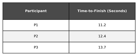
While we have a table with the time-to-finish for each participant, we might want to aggregate the data into a centrality measure in order to make a statement about the entire population, such as the mean time-to-finish for the race participants.
On average, it took the participants ~12.4 seconds to complete the 100 meter dash. However, there is a problem. In the race analogy we wait for all participants to cross the finish line before we calculate the mean. However, in many of the time-to-event scenarios we face in security, we analyze the data prior to all observations reaching the event.
To give you an example, it’s more like we measure the time until each participant crosses the finish line, but we stop measuring at the 13 second mark. In this scenario, our table will look a little different:
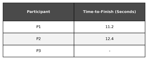
When we calculate the average, what do we do? We might decide the exclude those that did not finish the race while we were measuring. Let’s calculate the average, excluding participant 3:
We calculated a mean of 11.8 seconds, 0.6 seconds faster than the previous example. We could have any number of participants who were still sprinting at the 13 second mark and our mean would continue to be 11.8 seconds.
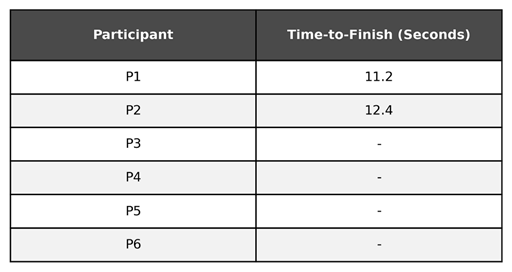
However, if we did not stop measuring at the 13 second mark and instead observed the time-to-finish for participants 3-6, the mean would likely be significantly higher. Saying it takes participants on average 11.8 seconds to complete the 100 meter dash in this scenario is misleading.
This is the core problem with time-to-event data, especially in security. We often don’t observe the start and event time for every observation. Whenever we decide to stop measuring, there will be some vulnerabilities that have yet to be patched, some alerts that have not been triaged, etc.
Censored Data
Censored data refers to an observation where the information about the time-to-event is incomplete, usually because the event did not occur within the study’s timeframe or the subject was lost to follow-up. Our 100 meter dash participants who had not yet completed the race when we stopped measuring are an example of censored data: we know that these participants took greater than 13 seconds to complete the race (because they were still sprinting when we stopped measuring), but we do not know how long they took. They could have finished in 13.1 seconds, or 130 seconds.
In security, we often encounter censored data when measuring the time to an event. In fact, the censoring problem is the primary reason we can’t use the mean.
For example, when measuring the efficiency of a Security Operations Center (SOC) in detecting and responding to security events, security teams may measure the following time-to-event data for an incident:
Time-to-Detect: The duration from the first activity of the incident to an alert/incident being raised to the SOC
Time-to-Resolve: The duration from the alert/incident being raised and the incident resolution
Note: Your SOC may define these differently. As long as you have a start and stop time defined, it doesn’t matter. I chose these definitions to keep it simple for this demonstration.
The security team pulls incident data from the prior week and starts the calculate the Mean Time-to-Detect (MTTD) and Mean Time-to-Resolve (MTTR).
Everything looks great when calculating the MTTD: The list of incidents all have a timestamp for when the incident was created in the SIEM, so they calculate the time to detect and average it. However, when they review the closed timestamps, there is an issue. Not all incidents were resolved last week, and as such, some of the incidents do not have a closed timestamp.
The security team could calculate the MTTR for only the incidents that were closed. However, as we saw in the race analogy, that will cause the metric to be misleading.
Despite the data being censored, the security team does know some information about the time-to-resolve for incidents that have not yet been resolved. They know that they took at least as long until the end of the measurement period. That knowledge should be included in the calculation, somehow…
Survival Analysis
The good news is that time-to-event data is a well researched domain of statistics, and one that has been solved for. We just don’t commonly use these tools in security measurement (yet).
Survival analysis is the statistical modeling of how much time elapses before an event occurs. Survival analysis can be used to model the time until almost any “event” which makes it an excellent application for a variety of time-to-event scenarios in security.
Subjects and Events
In survival analysis, you will see reference to subject(s). The subject is who/what we are measuring the duration of until it experiences the event. It’s important to note that the subject is not the same as the event being analyzed, but instead the subject experiences the event.
Let’s look at some examples inside and outside of the security domain:
We are analyzing how long a patient survives a critical medical condition after treatment is administered.
Subject: Patients
Event: Death
We are analyzing how long new tires last before being replaced.
Subject: Tires
Event: Replacement
We are analyzing how long software vulnerabilities remain in the environment until they are remediated.
Subject: Software vulnerabilities
Event: Remediation
We are analyzing how long it takes the organization to review a new vendor request for security requirements.
Subject: New vendor requests
Event: Vendor security determination
We are analyzing how quickly security incidents are detected.
Subject: Security incident
Event: Detection
Survival
Survival refers to the subject not experiencing the event. The term survival is used because survival analysis was originally developed for use in modeling patient survival from time of treatment until death (morbid, I know). In this scenario, the terms are pretty unambiguous: what is the probability a patient will survive until a specific time after treatment?
The techniques used in survival analysis, however, can be applied to any time to event data. We just have to reframe how we think about it. If survival means the subject does not experience the event:
When analyzing time-to-resolve of incidents, survival means the incident has not been resolved
When analyzing time-to-patch for software, survival means the software has not been patched
When analyzing the time-to-exploitation for vulnerabilities, survival means the vulnerability has not been exploited.
Depending on the event being analyzed, survival may be a good thing, or may be a bad thing (and in security it is often the latter, which can be a bit unintuitive).
Survival Time
Survival time is the duration (time) until a subject experiences the event. For example:
When analyzing time-to-resolve of incidents, an incident’s survival time is how long the incident took to be resolved.
When analyzing time-to-patch for software, a software’s survival time is how long it took to patch.
When analyzing the time-to-exploitation for vulnerabilities, a vulnerability’s survival time is how long it took to be exploited.
You can also think of this as the “time-to-x”. For example, calculating the Mean Time-to-Resolve (MTTR) is equivalent to calculating the mean survival time. But remember, we often do not know the survival time for all subjects, and as such the mean is misleading (we cannot use it).
The Survival Function: S(t)
The survival function is a mathematical function that expresses the probability that a subject’s survival time (the time elapsed before the event occurs) is greater than a specified time. In statistics, you will often see the survival function notated as S(t), where t = time.
For example, if we derive the survival function for MTTR, we could compute the probability of an incident to be resolved 10 minutes, 30 minutes, 2 hours, or even one week after the incident’s first activity (or another start time).
We might calculate these values as follows:
The survival function at time 10 minutes equals 0.7
The survival function at time 30 minutes equals 0.5
The survival function at time 2 hours equals 0.15
The survival function at time one week equals 0.02
Or said another way:
There is a 70% chance an incident is not resolved within 10 minutes.
There is a 50% chance an incident is not resolved within 30 minutes.
There is a 15% chance an incident is not resolved within 2 hours.
There is a 2% chance an incident is not resolved within one week.
The Cumulative Distribution Function: F(t)
The cumulative distribution function is a mathematical function that expresses the probability that a subject’s survival time (the time elapsed before the event occurs) is less than a specified time. You will often see the cumulative distribution function notated as F(t), where t = time.
This function is rather straightforward once you see the relationship. If we can interpret the survival function as “There is a 70% chance an incident is not resolved within 10 minutes”, we can also say “There is a 30% chance an incident is resolved within 10 minutes.”.
How do we get that? We subtract 70% from 100% to get 30%. In other words, it’s the inverse. That’s exactly how we can compute the cumulative distribution function given we know the survival function.
The Kaplan-Meier Estimator
We won’t know the true survival function, meaning we don’t know the exact probability of a subject to experience the event or not. Instead, we use statistical techniques to take the data we do have and estimate the survival function.
There are multiple techniques to do this, but a popular one is the Kaplan-Meier estimator (named after Edward Kaplan and Paul Meier who originally published the method in 1958).
Note: Using a Kaplan-Meier Estimator is as simple as running KaplanMeierFitter() in a statistical library such as Python’s Lifelines. However, I will briefly explain the math so you have a basic understanding of what’s happening under the hood.
The concept Kaplan and Meier introduced is relatively simple: break up the duration into intervals, calculate the probability of surviving during each interval, and then multiply them together. We multiply them together because a subject must survive each preceding interval. For example, in order for a subject to have a chance of surviving until day 20, they must first survive from day 0-1, then 1-2, then 2-3, and so on.
Let’s build a simple table to demonstrate this:
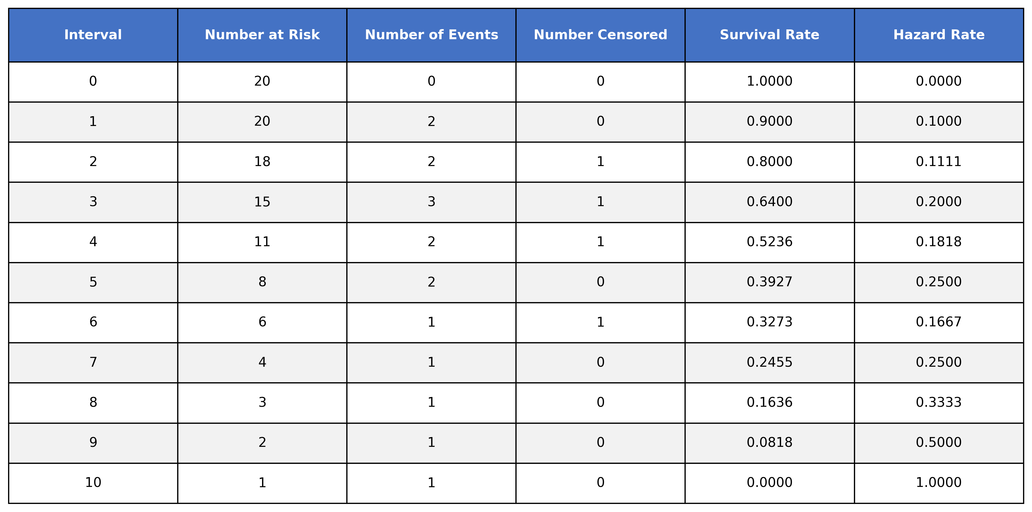
The table has the following columns:
Interval → The time intervals where events occurred in the dataset
Number at risk → The number of subjects at risk of experiencing the event (survivors) during the time interval
Number of events → The number of subjects who experienced the event during the time interval
Number censored → The number of subjects who were censored
Survival rate → The calculated survival rate
Hazard rate → The calculated hazard rate (we will cover this later)
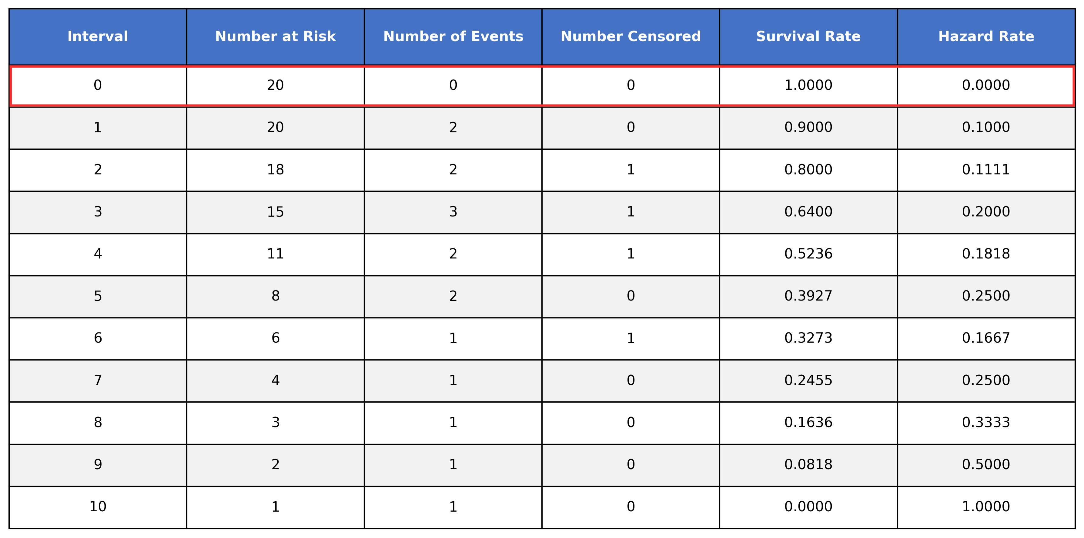
Looking at interval 0, we can see that all 20 subjects are at risk and no events were observed (this is usually assumed in survival analysis as time 0 is the exact time we started measuring). As such, all participants survived until interval 0 and the hazard rate is 0.
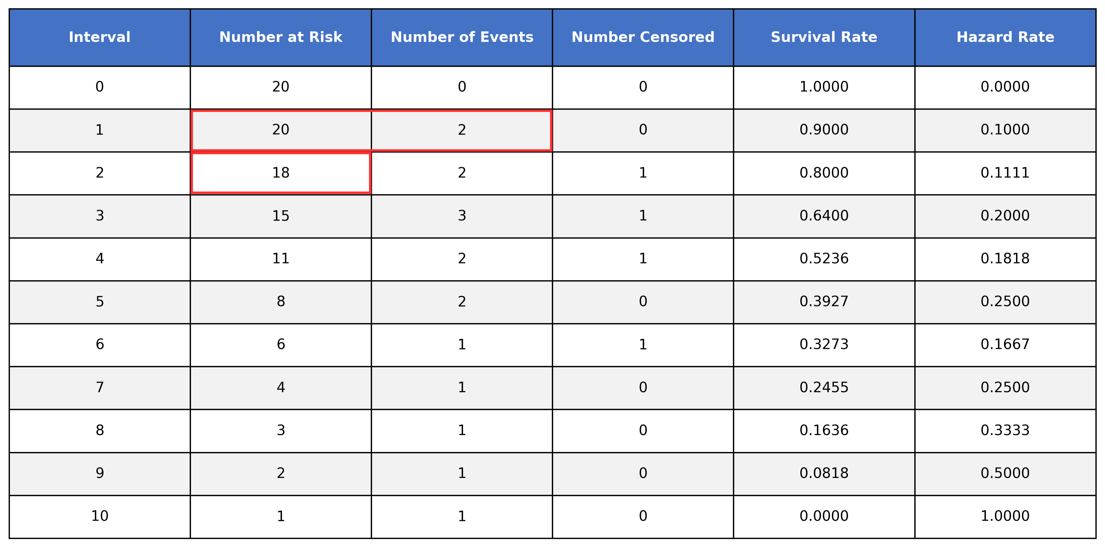
When we move down to time interval 1, we see that we have 20 subjects at risk. Of those 20 at risk, 2 of them experienced the event during this interval, while 18 of them survived the interval. Looking at time interval 2, we can see how the 18 survivors from interval 1 are at risk to experience the event during interval 2.
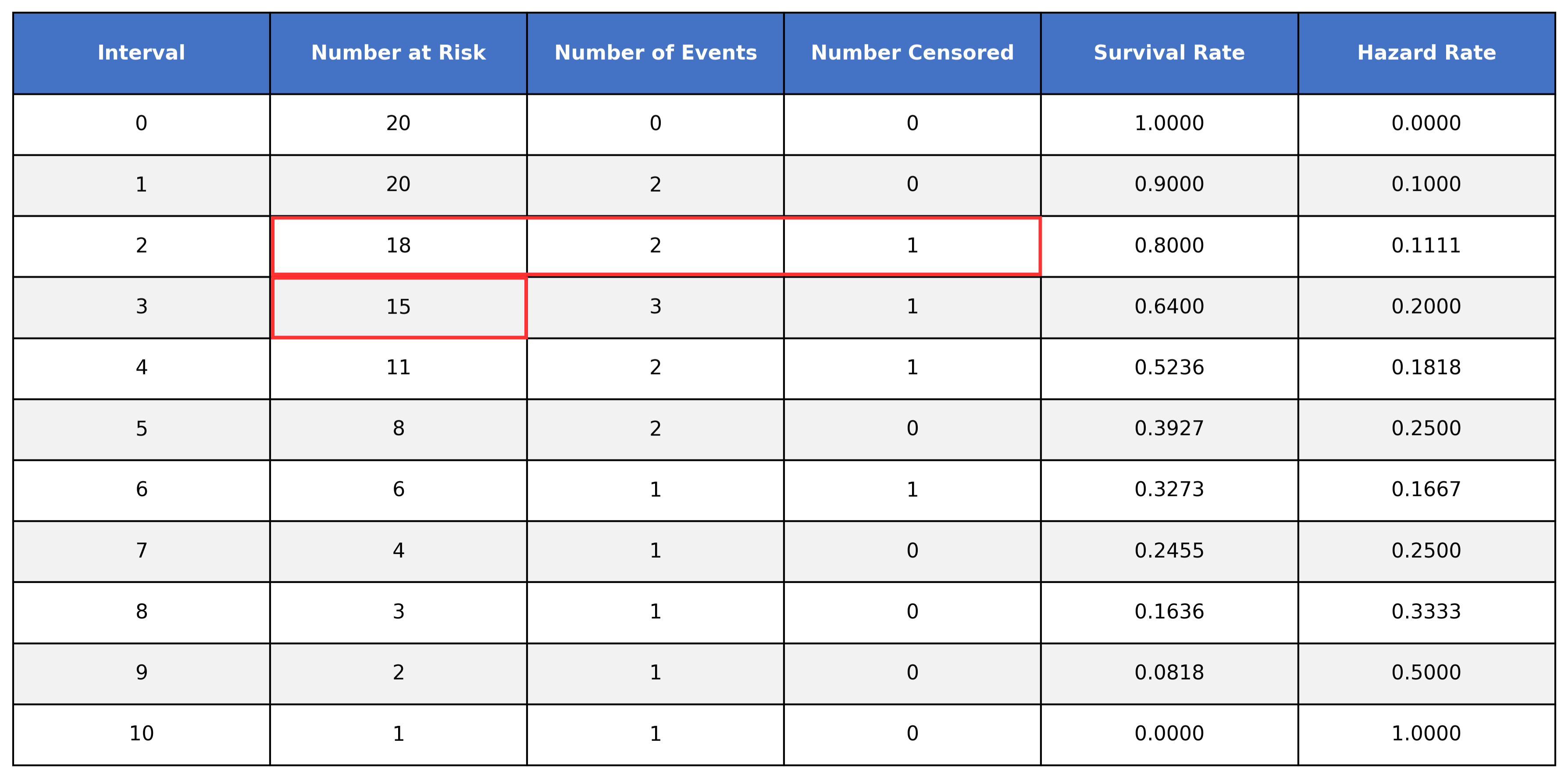
However, when looking at time interval 3, we get 16, not the listed 15:
In order to handle our censored data, we need to remove any censored subjects from the at risk pool:
To calculate the survival time, we take the number of at-risk subjects, subtract the number of events, and then divide it by the number of at-risk subjects. We then multiply that value by the value of the preceding time interval.
You don’t need to worry much about calculating the survival function by hand. What’s important to know is that we are calculating the probability a subject survives past the interval, accounting for censored subjects.
The Survival Curve
Looking at our previous table, you’ll notice we have a column for time and a column for the survival rate. Let’s keep just these two columns:
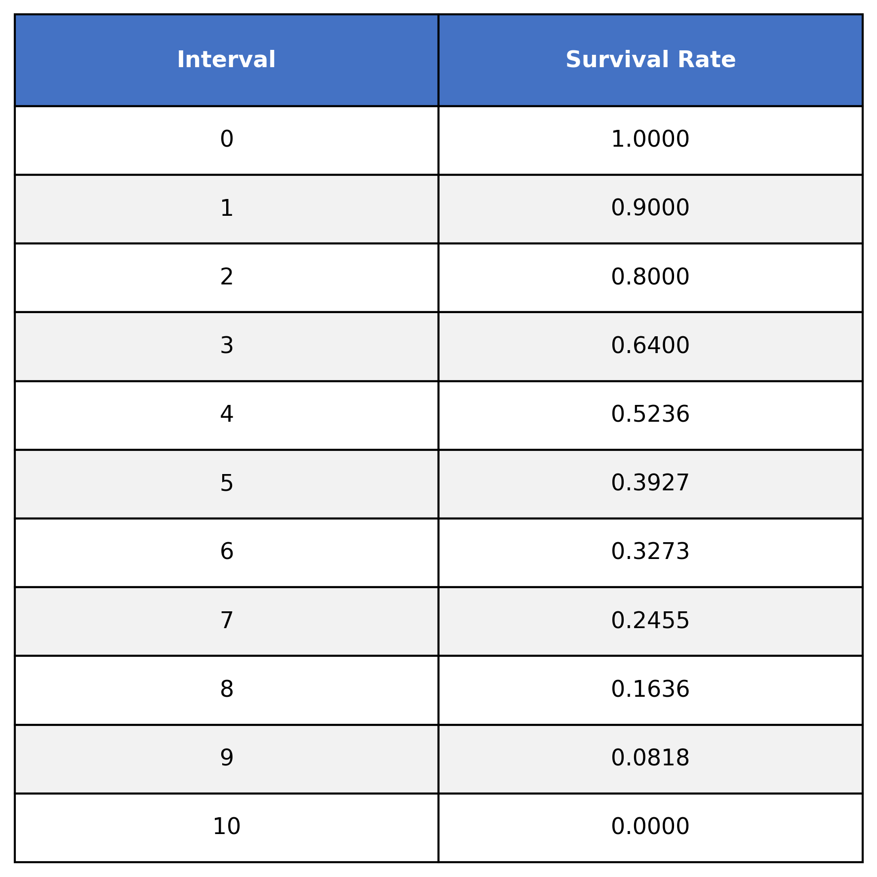
This table shows the survival function S(t), where t=time. For example:
S(0) = 1
S(1) = 0.9
S(2) = 0.8
S(3) = 0.64
etc.
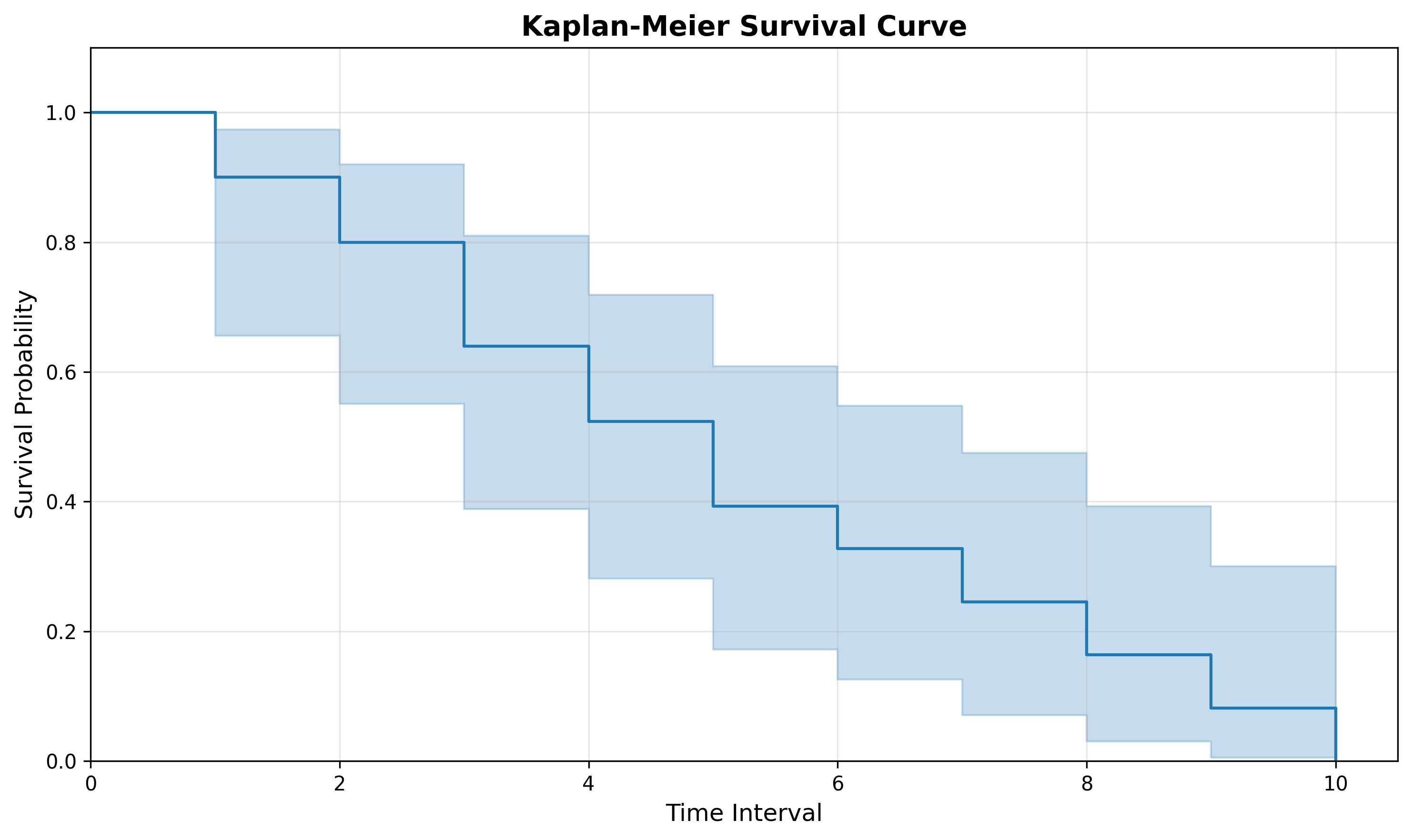
We can represent this graphically by plotting the interval column on the x-axis and survival rate on the y-axis:
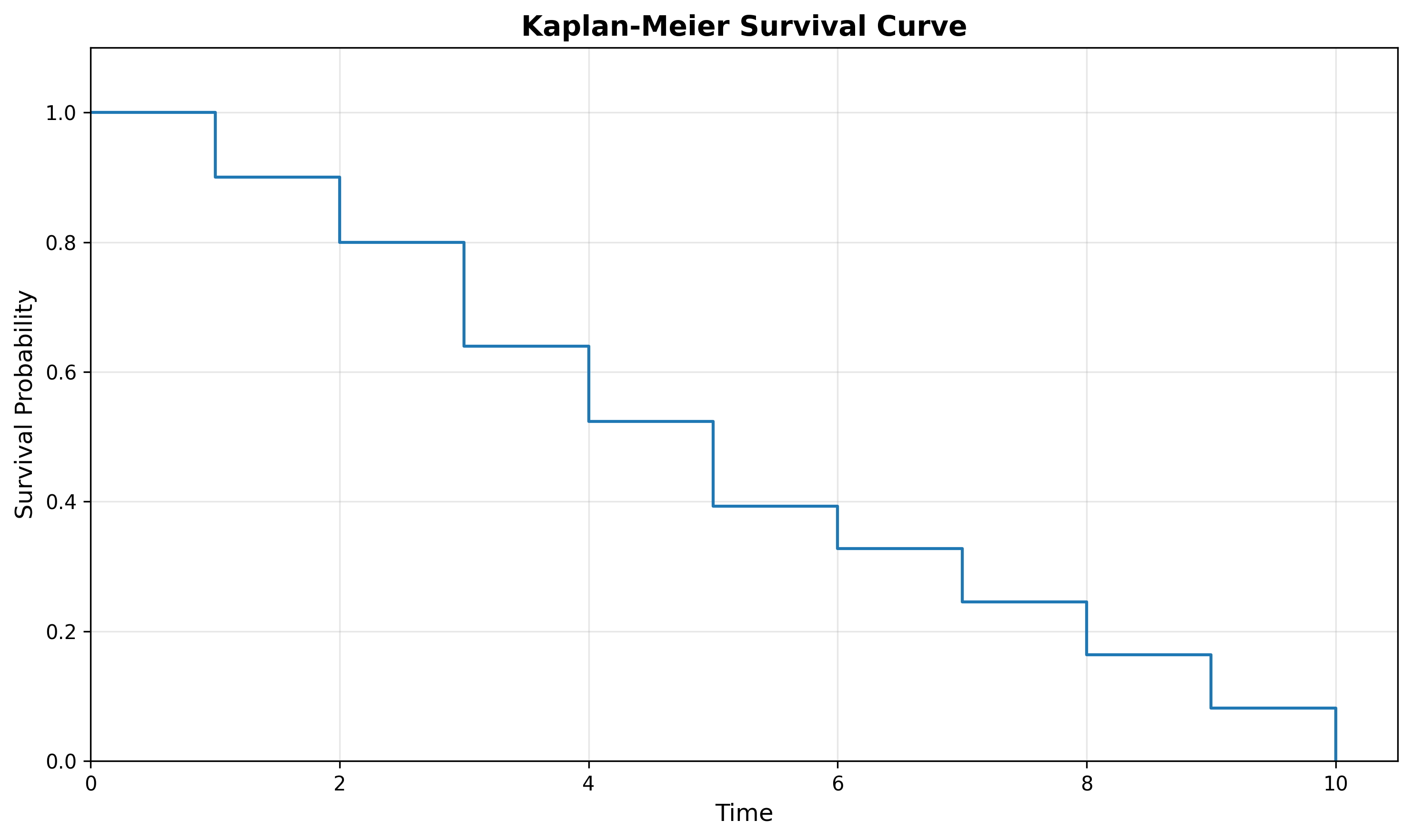
Notice that the above survival curve is a step-function (it looks like a set of stairs). Each vertical drop in the curve is where one or more events were observed. For example, events were observed at durations 1, 2, 3, 4, etc.
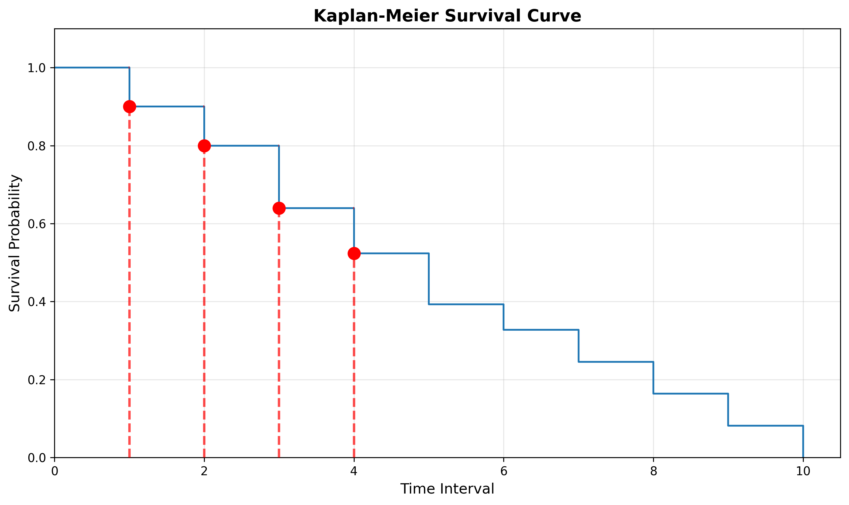
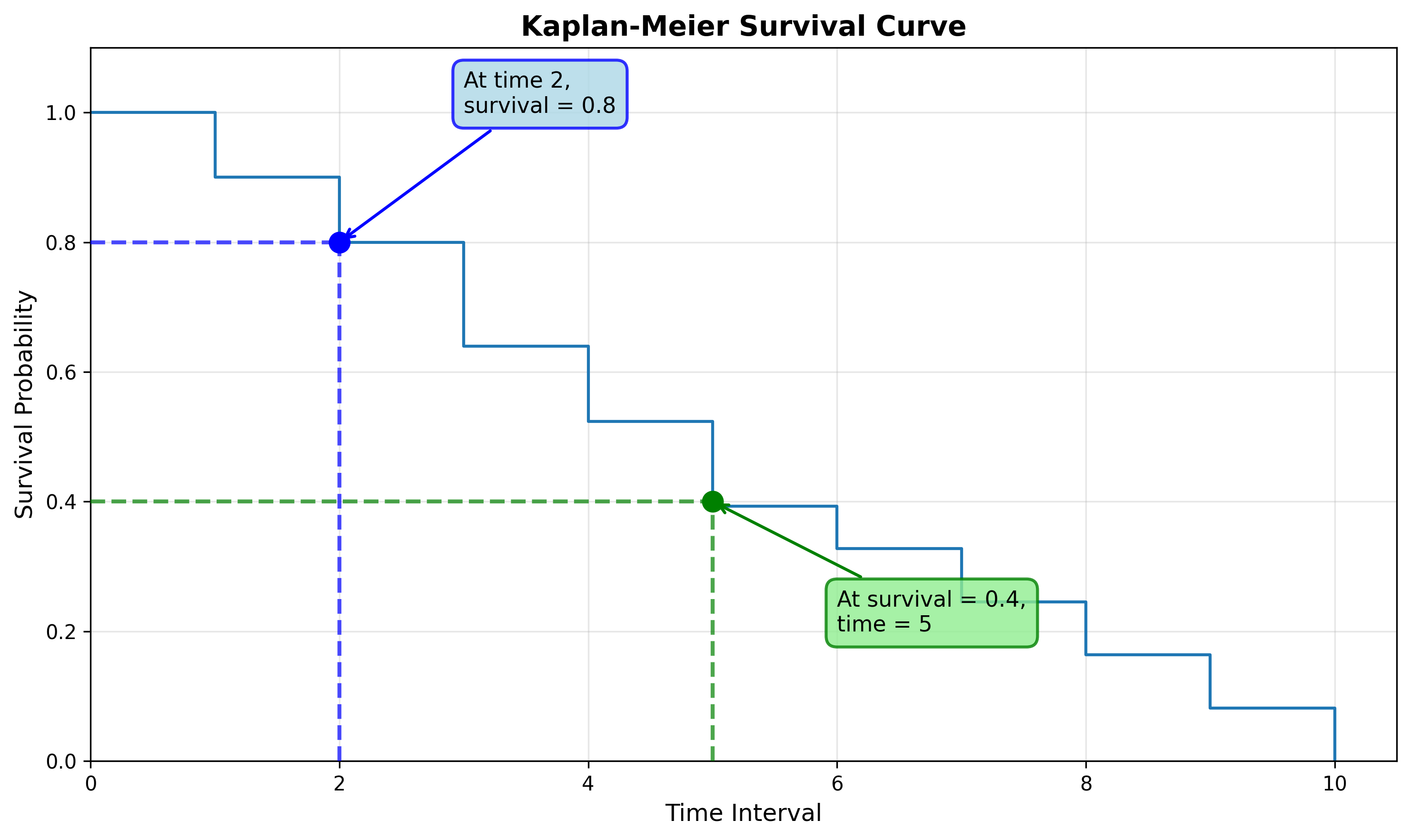
Reading the Survival Curve
We can read this curve in one of two ways:
Starting from the x-axis: What is the survival probability at time 2?
Starting from the y-axis: At what time is the survival probability 0.4?
Confidence Intervals
Remember that the Kaplan-Meier Estimator is estimating the survival function. Because we are estimating and don’t know the true curve, you’ll often see the curve plotted with confidence intervals (usually as a shaded region).
Confidence intervals essentially plot the upper and lower bounds of where we think the survival curve is at a specific time. Said another way, we are 95% confident the survival time at time t is within the shaded region.
Comparing Survival Functions
When analyzing time to event we data, you’ll likely want to compare times between time periods or groups. For example, we might want to compare the functions for incident resolution today from last quarter to understand how performance has changed over time. Or, we may want to compare the functions between groups, such as incident type or severity. There are multiple ways to do this with survival analysis.
Median Survival Time
Note: To calculate the median survival time we must have had at least 50% of subjects experience the event within the measurement period.
The median survival time is a good alternative to using the mean (such as Mean-Time-to-Resolve) as it provides a centrality measure for the dataset that accounts for censored subjects.
We can calculate the median survival time by looking at the time where the survival function equals 0.5 (50%). We can interpret this as, “50% of subjects will experience the event by the median survival time”. Or, given our example below, “50% of subjects will experience the event by time interval 5.”
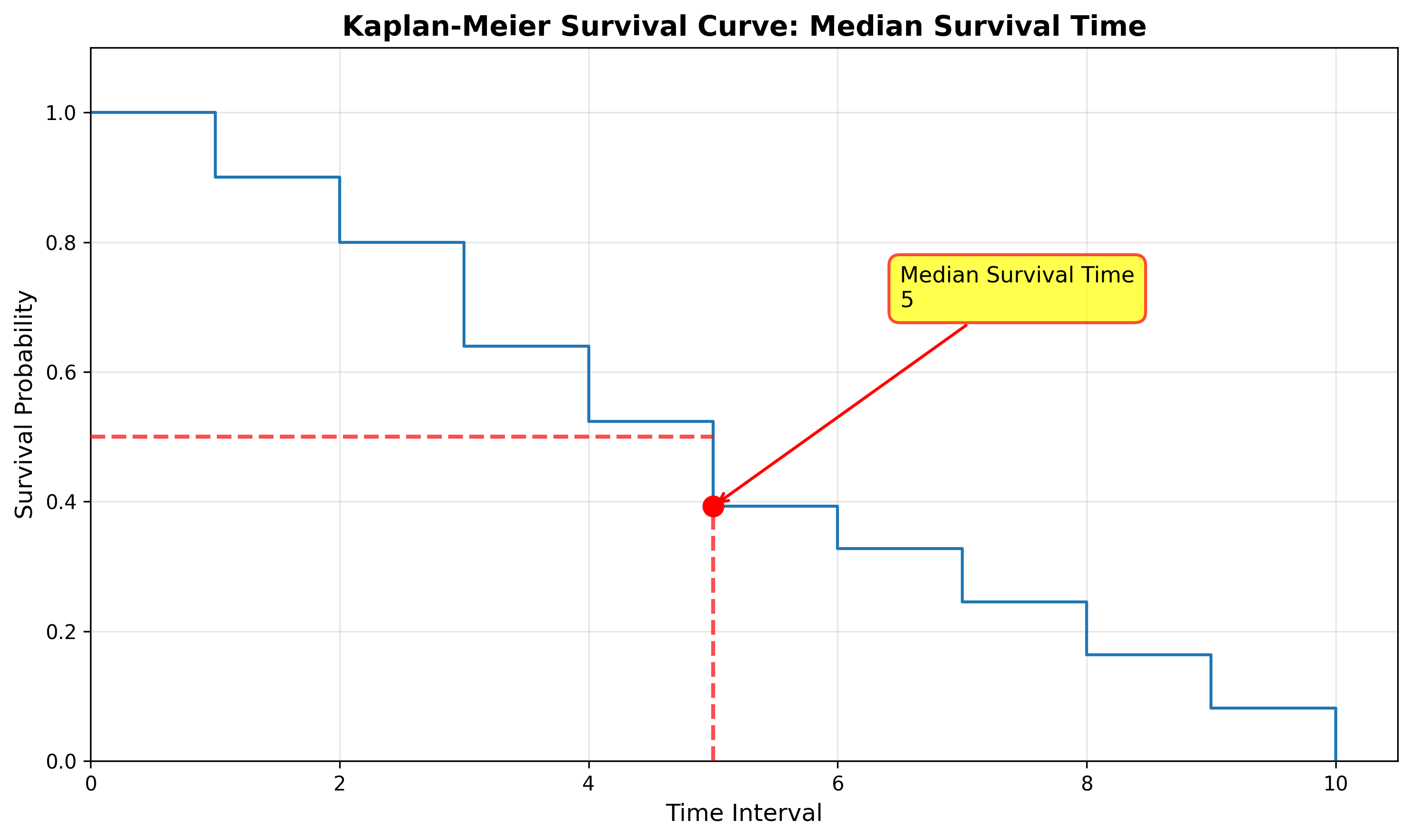
We can use the median survival time to compare against other groups (such as the median survival time for command and control incidents compared to malware) or compare the median survival time over time (such as the median survival time for Q1 vs Q2).
Restricted Mean Survival Time (RMST)
While we can’t use the mean due to censored data, we can use the Restricted Mean Survival Time (RMST). The RMST calculates the average survival time within a specified time period. For example, you could calculate the RMST from the baseline (time=0) up until time 10.
If we have the RMST for two curves using the same period, we can subtract them to find the area between the two curves:
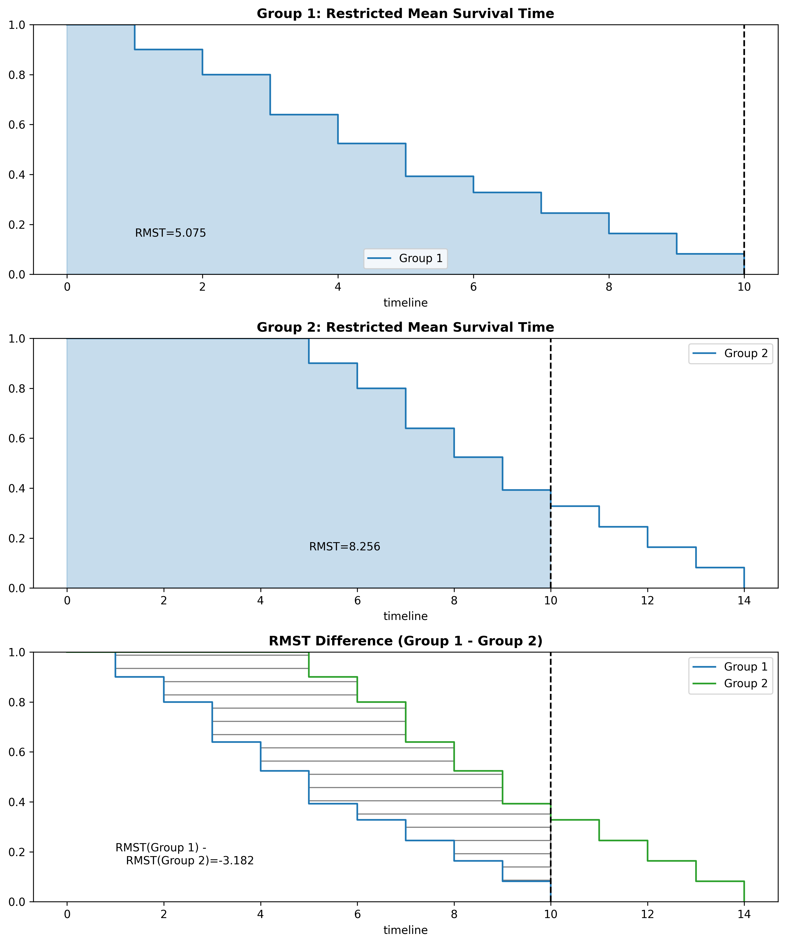
The most difficult part in using the RMST is selecting an appropriate time period to analyze. While I won’t go to in-depth on choosing a time period for the RMST, one method is setting the time period to whichever curve has the smallest maximum time period (which was used in the figures above). In some scenarios, there will be a time period to analyze that is significant (related to the problem being modeled). Regardless, when comparing values between two curves, ensure they are both using the same time period.
LogRank Test
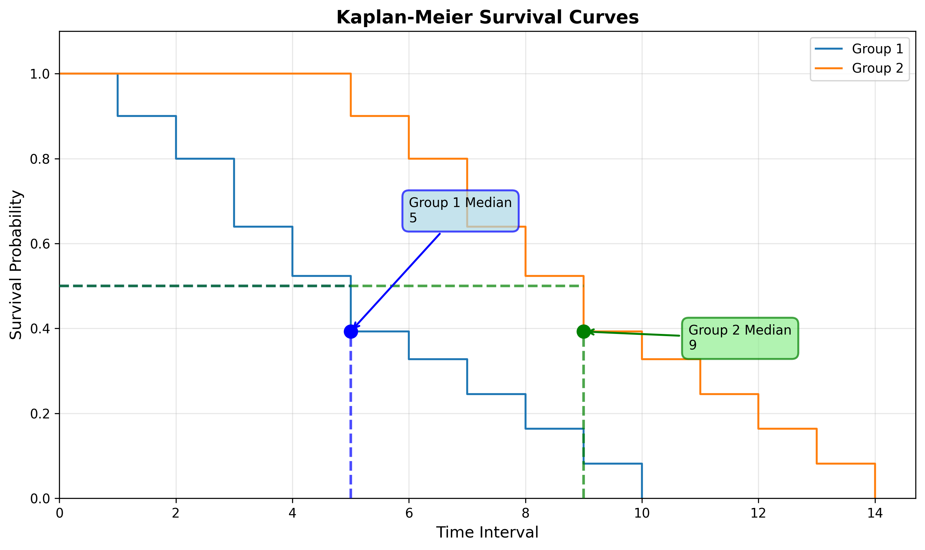
We may want to test if two survival functions are statistically different. For example, we may take a dataset and create two survival functions, one for the time-to-resolve for phishing incidents, and one for non-phishing incidents. When we plot the two curves they look like this:
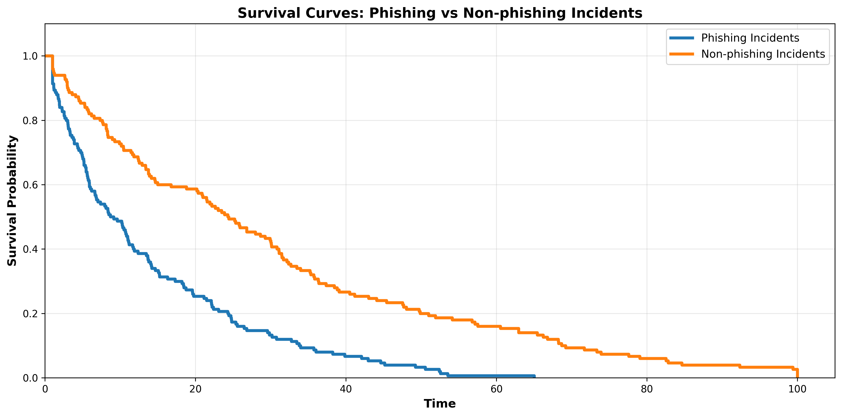
At first glance it appears that phishing incidents are in fact resolved faster than non-phishing incidents. Let’s quickly compare the median survival times:
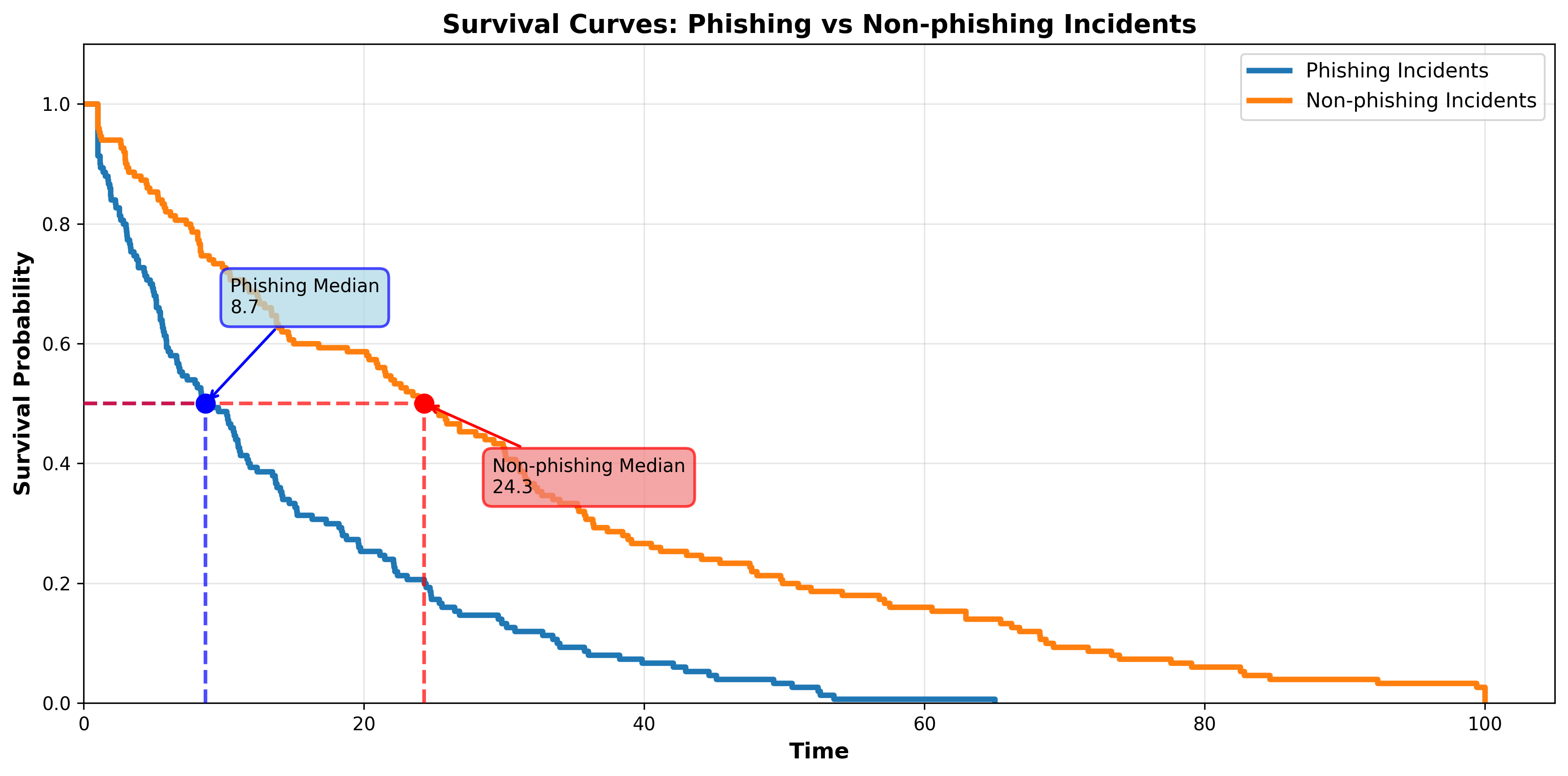
While it seems pretty clear that phishing incidents are resolved faster than non-phishing incidents, that won’t always be the case. To test if the curves are truly different (and not just caused by random chance) we use the LogRank Test.
The LogRank Test will return something called a p-value. The p-value is our indicator of statistical significance. If the p-value is less than 0.05, we can conclude that the two survival curves are in fact statistically different. However, if the p-value is equal to or greater than 0.05, we cannot conclude that the two curves are different.
The Hazard Function
The hazard function is a mathematical function that returns the instantaneous rate at which the event occurs at a specific time, given that it hasn’t happened before that time. In other words, the hazard function computes the risk of an event occurring at a specific time. You will often see the hazard function notated as h(t), where t = time.
The hazard rate is less intuitive to interpret then the survival probability. The biggest difference is that the hazard is not a probability, but a rate. For example, the speed your vehicle is traveling in miles per hour (mph) is a rate. If you are traveling at 60 mph, you would travel 60 miles within one hour assuming the rate did not change. In reality, however, your speed will change over time. You may be traveling at 40 mph in the city, then accelerate to 75 mph on the highway. Even during your travels your speed will fluctuate.
Just like mph, our hazard rate is a rate of units/time:
Miles per hour
distance/time
Hazard rate
events/time
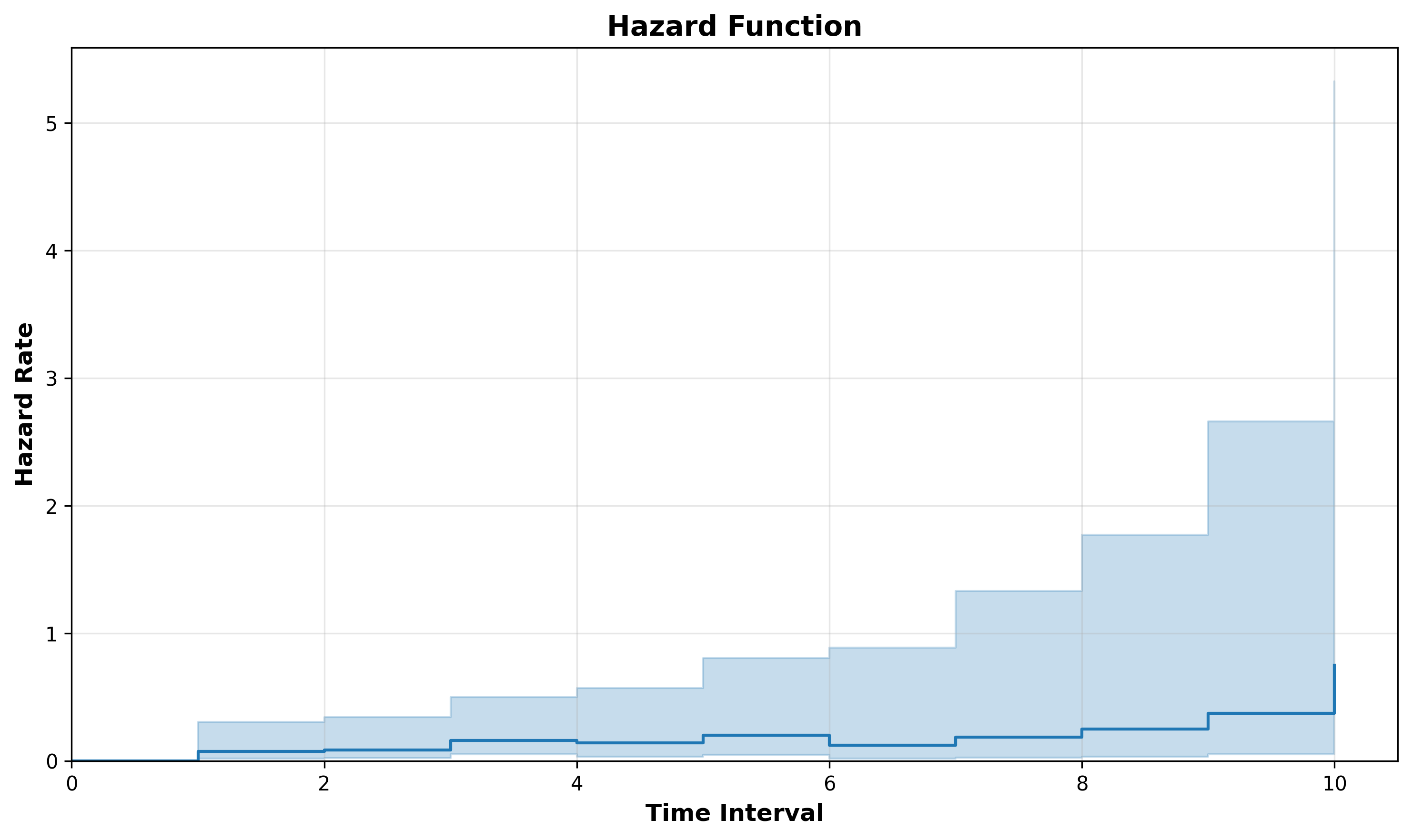
We can visualize the hazard function by plotting the hazard rate on the y axis and time on the axis:
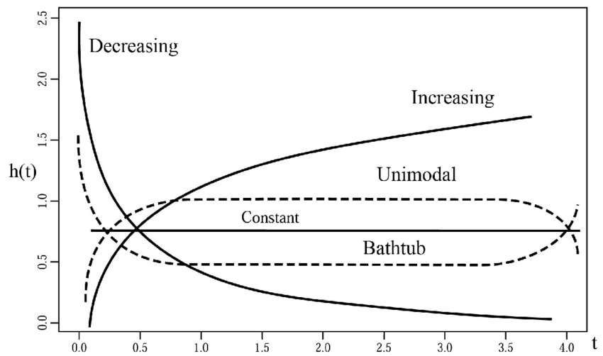
Hazard Function Shapes
How the hazard function changes over time is particularly of interest. For example, if the hazard function increases over time, that means the likelihood of the subject experiencing the event increases faster as it ages. On the other hand, if the hazard function decreases over time, that means the likelihood of the subject experiencing the event decreases as it ages.
1. Increasing Hazard Rate
An increasing hazard function means the conditional probability of the event occurring increases as time passes.
Example: As a machine gets older, the chance of it failing in the next hour is higher than it was when the machine was new.
2. Decreasing Hazard Rate
A decreasing hazard function means the conditional probability of the event occurring decreases as time passes.
Example: If a transplant patient survives the first 48 hours, their risk of immediate complication often drops significantly.
3. Constant Hazard Rate
A constant hazard function means the conditional probability of the event is not changed over time.
Example: The object doesn’t “age” in terms of its risk; it is just as likely to fail today as it is a year from now.
Let’s think through the expected hazard function for different scenarios:
Scenario 1
We are analyzing the duration from when a software patch is available until the affected software is patched by the organization.
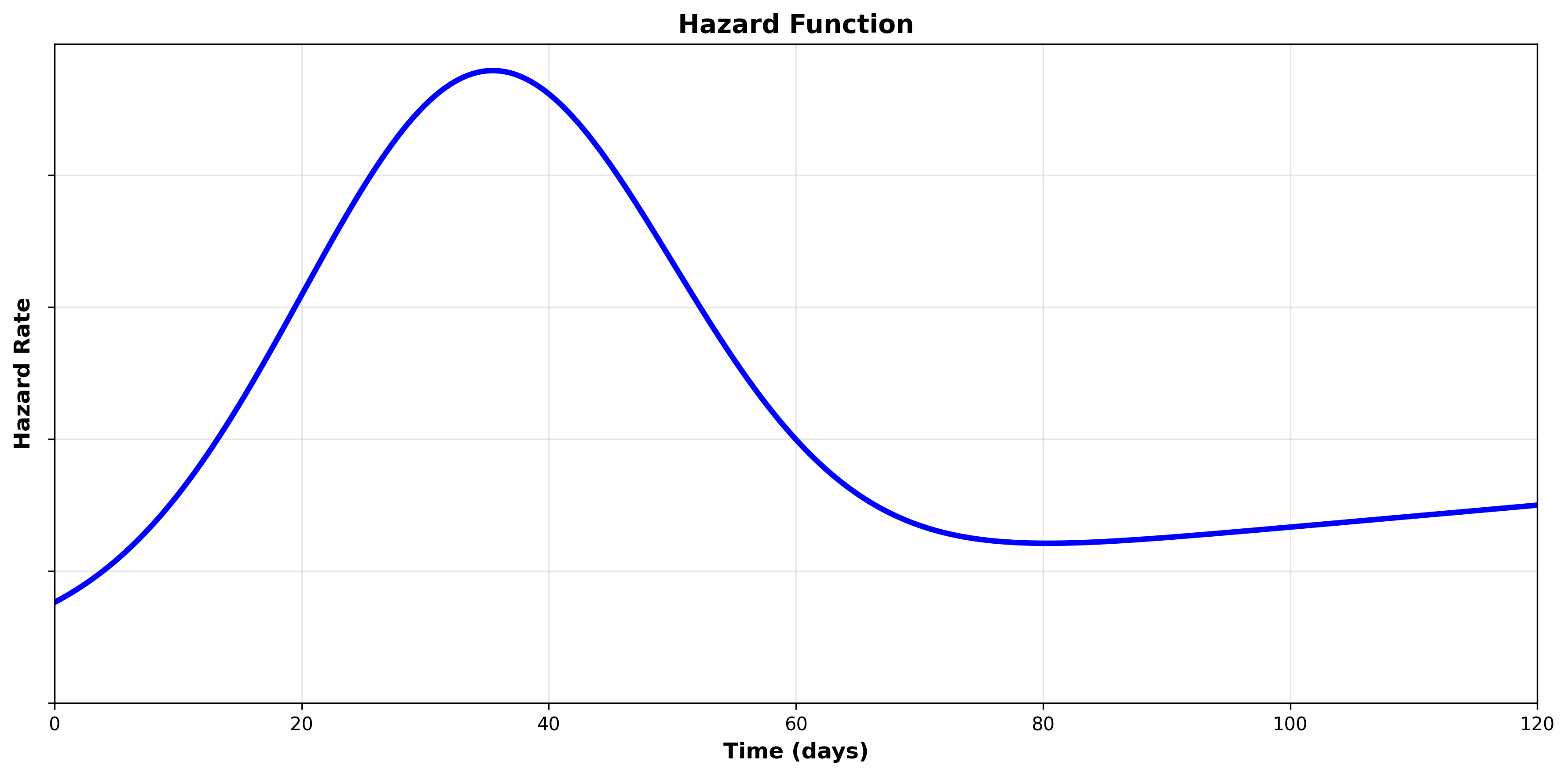
We may expect that the hazard increases over time in the beginning as the organization prioritizes, schedules, tests, and eventually rolls out software patches.
However, once the software has survived long enough without being patched, the hazard may fall significantly, as the organization has either accepted the risk and will not patch or is not aware/managing patching of the software entirely.
Scenario 2
We are analyzing the duration from employee leave until assets (such as a laptop) have been retrieved.
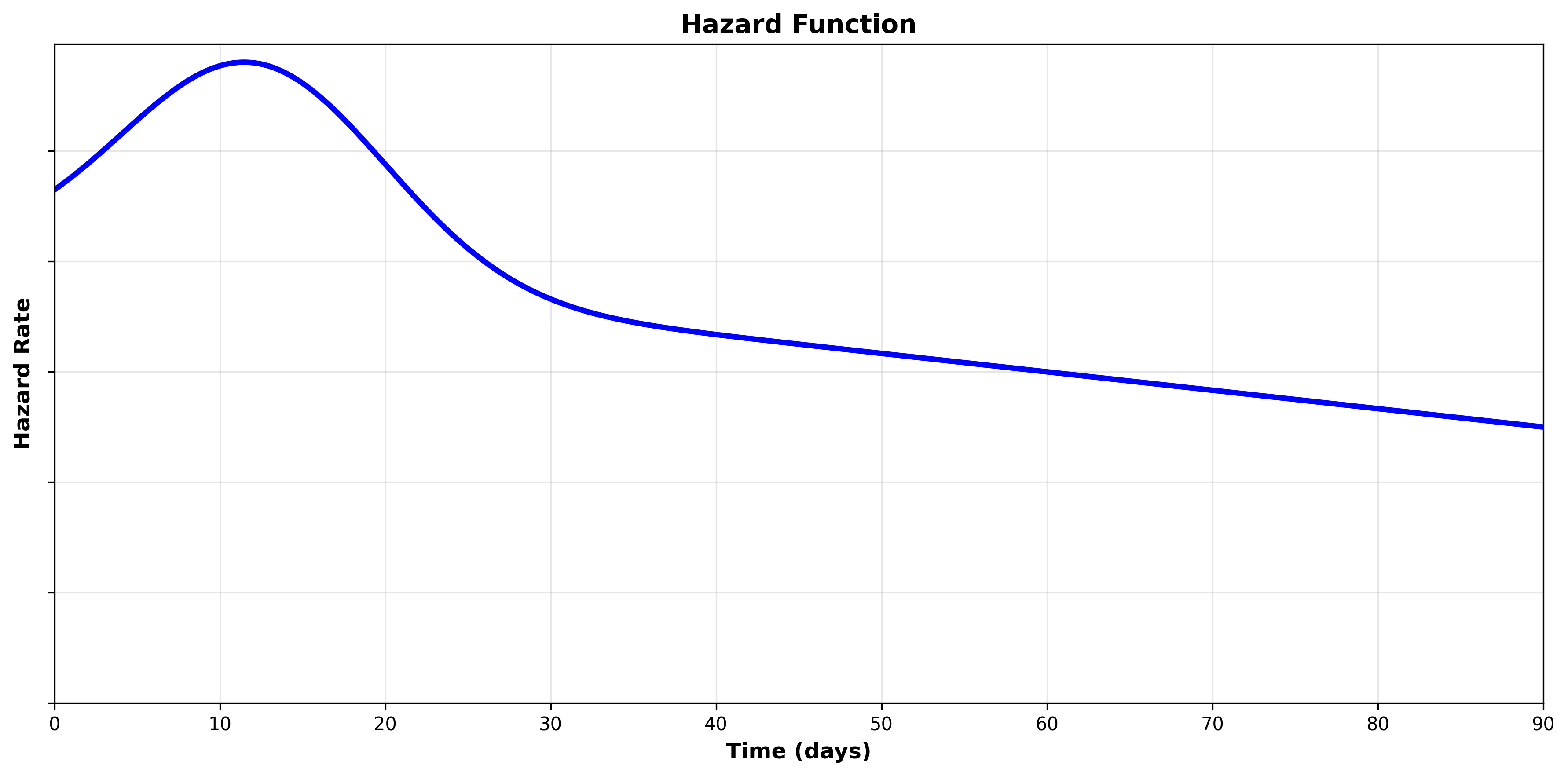
We may expect that the hazard is relatively high in the beginning as many employees are in the office on their last day to return assets.
Some employees are remote, and as such the hazard will continue to climb over the short term as assets are retrieved.
Eventually, the hazard will fall when enough time has passed without successful retrieval, causing the organization to instead implement compensating controls such as remotely wiping the devices or pursuing legal action.
Scenario 3
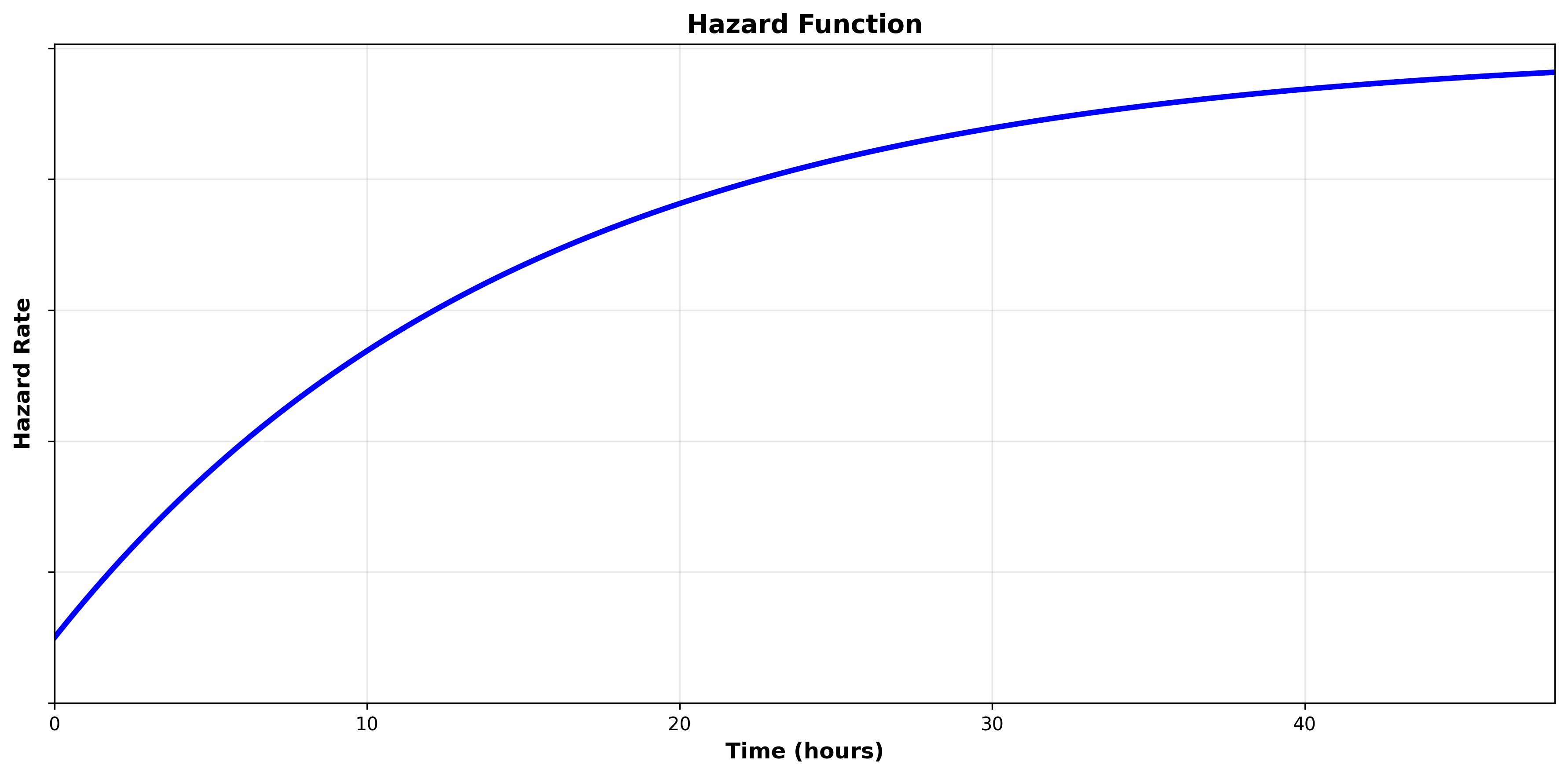
We are analyzing the duration from an alert being raised in the SOC until it is resolved.
We may expect that the hazard starts low when the alert is first triggered, and the likelihood of the alert being resolved continues to increases over time.
Cumulative Hazard Function
The cumulative hazard function calculates the total accumulated risk of experiencing the event over time. While the hazard function calculates the risk at a specific time, the cumulative hazard function calculates the total risk of the current time and the time that has already passed.
Think of it this way: The hazard function assumes that the subject has already survived until a specific point in time, so, given that fact, what does that tell us about their risk of experiencing the event now? In our example of retrieving assets after employee leave, the fact that the assets haven’t been retrieved in 90 days means they less likely to be retrieved right now than they were in the first 7 days.
The cumulative hazard function, on the other hand, takes into account that for a subject to survive until a specific time, they must also face the risk of every time point before that. In our example of retrieving assets after employee leave, while the rate of retrieval may be low at 90 days, most assets are retrieved prior to 90 days as the likelihood an asset is retrieved within 90 days is very high.
We can visualize the cumulative hazard function by plotting the cumulative hazard on the y-axis and time on the x-axis:
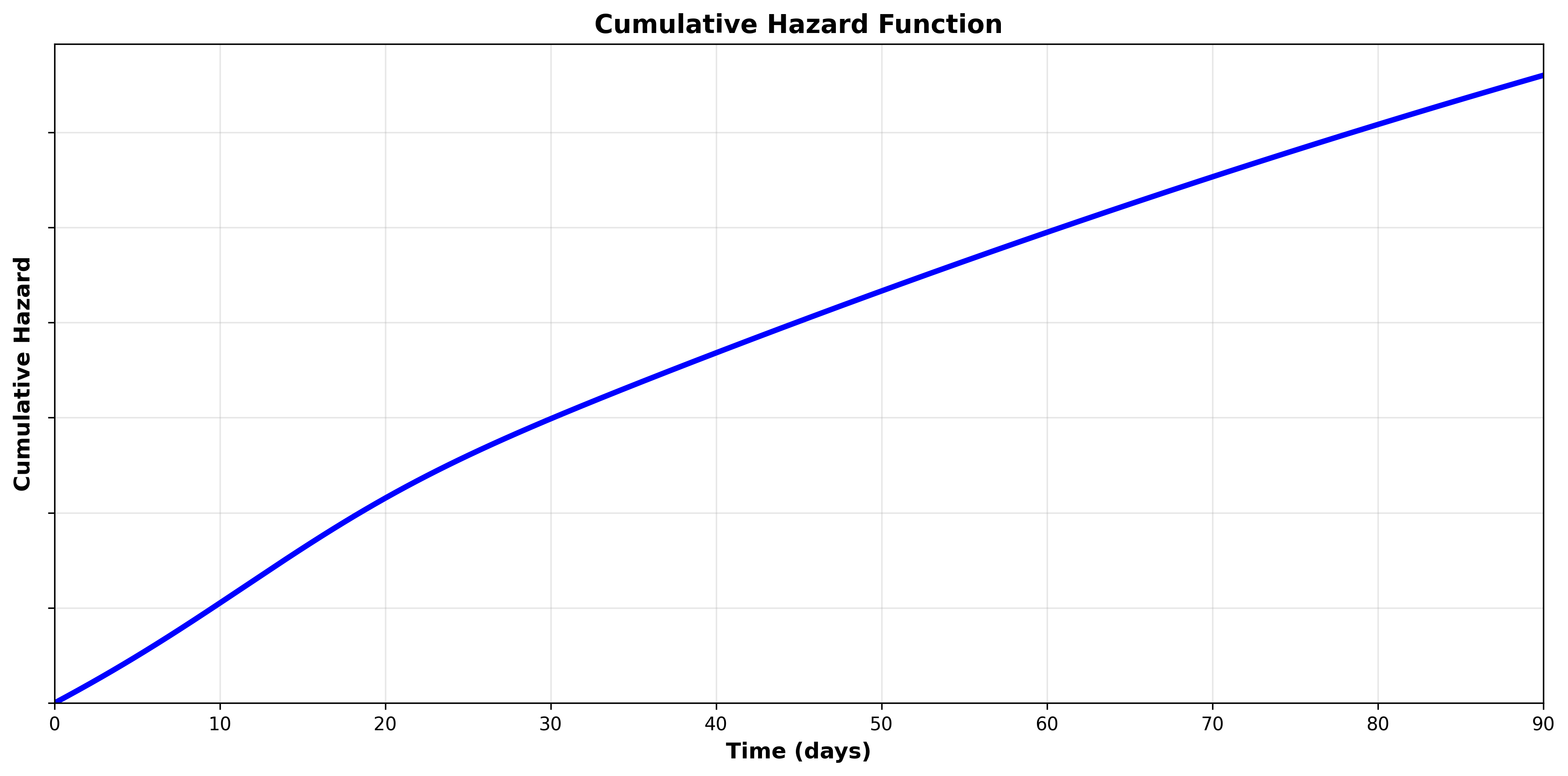
Because the cumulative hazard function is cumulative (integrates the hazard function), it is always positive and always increasing. The hazard function tells us the rate at which the cumulative hazard function changes (the derivative). Let’s look at the hazard function to see the relationship:

We can see that the hazard starts high and then decreases over time. We can see the same behavior in the cumulative hazard function, where the rate of change is faster in the beginning and then slows down.
Partitioned Survival Analysis
So far, we have been analyzing a single duration. However, in many security applications of survival analysis there are multiple steps or phases we are analyzing. One example of this would be incident lifecycles in a SOC. In a SOC, there are multiple discrete phases. One way to organize these phases is detection, triage, investigation, and response:
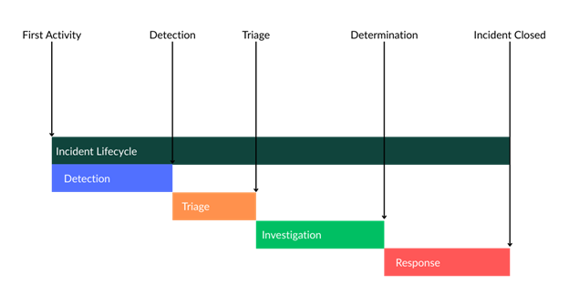
We could perform survival analysis on each stage independently by shifting the start time for each phase as the event time for the previous:
Detection
Start = First Activity
Event = Detection
Triage
Start = Detection
Event = Triaged
Investigation
Start = Triaged
Event = Determination
Response
Start = Determination
Event = Closure
In this case, we would get four distinct survival curves that models that phase’s survival time. However, we can also model the entire process by setting the start time for each phase as the time the subject becomes at risk for the first phase. This is called partitioned survival analysis. For example:
Detection
Start = First Activity
Event = Detection
Triage
Start = First Activity
Event = Triaged
Investigation
Start = First Activity
Event = Determination
Response
Start = First Activity
Event = Closure
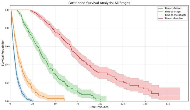
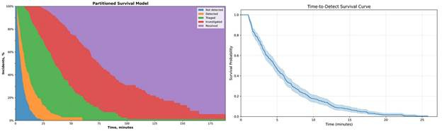
We can visualize this partitioned model on a chart:
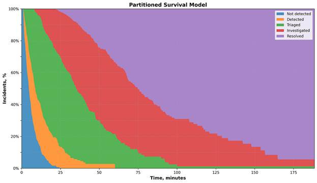
When analyzing portioned models, it can be useful to plot it as a stacked area chart, as the area between the curves can be thought of the subjects within those states:
When looking at a specific duration, we can see the proportion of incidents in each state:
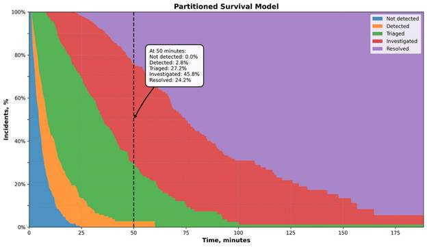
50 minutes after the incidents’ first activity:
100% are detected
97.2% are triaged
70% are investigated
24.2% are resolved
Note that in the partitioned model we are looking at the lifecycle as a whole. Each subsequent step’s duration is dependent on the duration of the previous steps since each steps’ duration is calculated using the incident’s first activity as the start time.
This is important when comparing survival curves in a partitioned model. We might see an improvement in incidents being resolved faster from Q1 to Q2, but this improvement could be due to faster detection, triage, investigation, and/or investigation. In order to identify improvement in a specific step, we need to measure the area between the curves (the shaded areas on our stacked area chart). The area between the curve is equivalent to the individual survival curve if analyzed independently.
Conclusion
Survival analysis is one of the most transformative statistical tools the security professional can learn. Throughout security you will encounter time-to-event problems, and all to often we use the wrong statistical techniques (such as the mean) to measure them.
While survival analysis can seem complicated at first, once you have the basics down you will be much better equipped to answer key time-to-event questions, improve decision making, and translate findings into easy to understand statements.
But this is just the beginning of survival analysis. While this guide will arm you with the tools needed to answer most questions, there is a big world of advanced techniques that build off this foundation.